Decided to publish the code from yesterday’s example, though wordpress only allows for certain somewhat odd file types to be shared, so I am just copy/pasting below. There are 5 functions, and as usual, you save each to the same folder in MATLAB, open that folder, and then typing
>>billiardgame3(25,10,15,20)
will generate a 3-dimensional billard game with 25 balls of masses between 0 and 10, speeds between 0 and 15 bouncing for 20 seconds, then play this. It also returns the position vectors [X,Y,Z] associated with this. I’d be glad to also publish the 2-dimensional version of this, though it should not be too hard to wade through my code and cut it down to two dimensions.
function [v1n,v2n] = collide3(m1,m2,v1,v2)
%solves the conservation of velocity and momentum for two balls of mass m1
%and m2 colliding at velocities v1 and v2, and returns their new
%velocities.
C1 = (m1-m2)/(m1+m2);
C2 = (2*m2)/(m1+m2);
C3 = (2*m1)/(m1+m2);
v1n = C1*v1+C2*v2;
v2n = -C1*v2+C3*v1;
end
function [A,W] = collisions3(X,Y,Z,rad,w,l,h)
%takes vectors X, Y, and Z where each entry contains the x- or y-position of
%a billiard ball and returns an n x 2 matrix A containing the indices where
%there is a collision (assuming balls have radius rad),
%and a matrix W containing the indices of which balls collided with walls
%in a w x l x h rectangle
C = X>=w; %oddly, I can’t find a way to make this code nicer. Checks collisions with walls
C = +C;
D = Y>=l;
D = +D;
E = X<=0;
E = +E;
F = Y<=0;
F = +F;
G = Z>=h;
G = +G;
H = Z<=0;
H = +H;
C = C+D+E+F+G+H;
for j = 1:length(C)
if C(j) > 0
W = [W;j];
end
end
X = ones(length(X),1)*X;
Y = ones(length(Y),1)*Y;
Z = ones(length(Z),1)*Z;
B = sqrt((X-X.’).^2+(Y-Y.’).^2+(Z-Z.’).^2); %a matrix whose (i,j)th entry is the distance between particle i and particle j
B = B<rad;
A = [];
for j = 1:size(B,2)
for k = 1:j-1
if B(k,j)==1
A = [A;k,j];
end
end
end
end
function [X,Y,Z] = billiards3(w,l,h,M,vx,vy,vz,X0,Y0,Z0,T,rad,tstep)
%simulates billiards with elastic collisions on a w x l billiards table. M
%should be a vector recording the (positive) masses of the billiard balls
%(the function will create as many balls as the length of M). vx, vy, X0,
%Y0 will similarly be vectors giving the initial x and y velocities of each
%billiard ball, and then initial positions. The program runs for T seconds
%with time step tstep. A reasonable setup is
%billiards(9,4.5,randi(10,1,9),3*rand(1,9),3*rand(1,9),.5+randi(8,1,9),.4+ran
%di(4,1,9),5,.2,.01)
X = zeros(floor(T/tstep),length(M)); %initialize the three position arrays, one column per particle
Y = zeros(floor(T/tstep),length(M));
Z = zeros(floor(T/tstep),length(M));
X(1,:) = X0; %set initial position
Y(1,:) = Y0;
Z(1,:) = Z0;
for k = 2:floor(T/tstep)
tryxpos = X(k-1,:)+tstep*vx; %here we check if any collisions will happen in the next step
tryypos = Y(k-1,:)+tstep*vy;
tryzpos = Z(k-1,:)+tstep*vz;
[A,W] = collisions3(tryxpos,tryypos,tryzpos,rad,w,l,h);
for j = 1:size(A,1)
[vx(A(j,1)),vx(A(j,2))] = collide3(M(A(j,1)),M(A(j,2)),vx(A(j,1)),vx(A(j,2))); %avoiding collisions with particles
[vy(A(j,1)),vy(A(j,2))] = collide3(M(A(j,1)),M(A(j,2)),vy(A(j,1)),vy(A(j,2)));
[vz(A(j,1)),vz(A(j,2))] = collide3(M(A(j,1)),M(A(j,2)),vz(A(j,1)),vz(A(j,2)));
end
for j = 1:length(W)
if tryxpos(W(j)) >= w || tryxpos(W(j))<=0 %avoiding collisions with walls
vx(W(j)) = -vx(W(j));
elseif tryypos(W(j))>=l || tryypos(W(j))<=0
vy(W(j)) = -vy(W(j));
elseif tryzpos(W(j)) >=h || tryzpos(W(j))<=0
vz(W(j)) = -vz(W(j));
end
end
X(k,:) = X(k-1,:)+tstep*vx;%updating the position with the “fixed” velocity vectors
Y(k,:) = Y(k-1,:)+tstep*vy;
Z(k,:) = Z(k-1,:)+tstep*vz;
end
end
function billiardplayer3(X,Y,Z,ptime,w,l,h)
%a program for visualizing billiard movement in 3 dimensions.
figure(1)
axis equal
%maxwindow
for j = 2:size(X,1)
%color the first particle red
plot3(X(j,1),Y(j,1),Z(j,1),’ro’,’MarkerFaceColor’,’r’)
hold on
%keep the rest of the particles blue circles
plot3(X(j,2:size(X,2)),Y(j,2:size(Y,2)),Z(j,2:size(Z,2)),’o’)
hold off
axis([0 w 0 l 0 h])
grid on
pause(ptime)
end
hold on
%draw the path of the first particle
plot3(X(:,1),Y(:,1),Z(:,1),’k’,’LineSmoothing’,’on’)
end
function [X,Y,Z] = billiardgame3(N,massmax,vmax,T)
%generates and plays a game of billiards with N randomly placed billiard
%balls on a table. The balls have random mass between 0 and massmax,
%velocity between 0 and vmax, and plays for T seconds, with timestep .01.
w = 9;
l = 4.5;
h = 4.5;
M = massmax*rand(1,N);
vx = 2*vmax*rand(1,N)-vmax;
vy = 2*vmax*rand(1,N)-vmax;
vz = 2*vmax*rand(1,N)-vmax;
X0 = w*rand(1,N);
Y0 = l*rand(1,N);
Z0 = h*rand(1,N);
rad = 0.2;
tstep = 0.01;
[X,Y,Z] = billiards3(w,l,h,M,vx,vy,vz,X0,Y0,Z0,T,rad,tstep);
billiardplayer3(X,Y,Z,0.01,w,l,h)
end
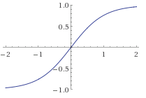
![The [activation] function sigma.](https://colindcarroll.wordpress.com/wp-content/uploads/2012/12/logistic.gif?w=640)


 with standard metric) is defined by
  . So the unit ball in Euclidean space is the collection of points of distance less or equal to one from, say, the origin. If you think I am being overly careful with this definition, you’re right!
 , and
, and  . So the volumes are getting bigger, and maybe we have a good question on our hands. But now what’s the volume of a four dimensional sphere?
 ,
, is the
  for integers n. Then, for even dimensions,
 .
.
 .
.


