[NOTE: At the end of editing this, I found that the substitution used below is famous enough to have a name, and for Spivak to have called it the “world’s sneakiest substitution”. Glad I’m not the only one who thought so.]
In the course of working through some (very good) material on neural networks (which I may try to work through here later), I noticed that it was beneficial for a so-called “activation function” to be able to be written as the solution of an “easy” differential equation. Here by “easy” I mean something closer to “short to write” than “easy to solve”.
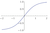
![The [activation] function sigma.](https://colindcarroll.wordpress.com/wp-content/uploads/2012/12/logistic.gif?w=640)
The [activation] function sigma.

and

One might observe that these satisfy the equations
and


By invoking some theorems of Picard, Lindelof, Cauchy and Lipschitz (I was only going to credit Picard until wikipedia set me right), we recall that we could start from these (separable) differential equations and fix a single point to guarantee we would end up at the functions above. In seeking to solve the second, I found after substituting cos(u) =τ that
and shortly after that, I realized I had no idea how to integrate csc(u). Obviously the internet knows (substitute v = cot(u) + csc(u) to get the integral being –log(cot(u)+csc(u))), which is a really terrible answer, since I would never have gotten there myself.


Not the right approach.
Instinctually, I might have tried the approach to the right, which gets you back to where we started, or by changing the numerator to cos2x+sin2x, which leads to some amount of trouble, though intuitively, this feels like the right way to do it. Indeed, eventually this might lead you to using half angles (and avoiding integrals of inverse trig functions). We find
Avoiding the overwhelming temptation to split this integral into summands (which would leave us with a cot(u)), we instead divide the numerator and denominator by sin2(u) to find
Now substituting v = tan(u/2), we find that dv = 1/2 (1+tan2(u/2))du = 1/2(1+v2)du, so making this substitution, and then undoing all our old substitutions:


The function tau we worry so much about. Looks pretty much like sigma.
Using the half angle formulae that everyone of course remembers and dropping the C (remember, there’s already a constant on the other side of this equation), this simplifies to (finally)


Phew.

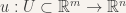
 (note to impressionable readers: the function defined below is not quite the gradient):
 , which takes a point in the domain, a direction in the domain, and returns the vector in the range. The idea being that if you had a map, knew where you are and in which direction you wished to travel, then the gradient should tell you what 3-dimensional direction you would head off in.
 .
. .
.
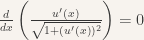
 is
is  . Notice that in order to write down this equality, we already named our solution u. But just working from this equation, we can deduce a number of qualities that any solution must have: u is infinitely differentiable and, restricted to any compact set, attains its maximum and minimum on the boundary of that set. Such properties quickly allow us to narrow down the possibilities for solutions to problems.
")

 which is convex and where F(t) = 0 only when t = 0. Recall that for a real valued function, convex means that every secant line lies above the curve. So far, so good. Such a function might serve as a measure of how alike two functions are: rather than looking at (for example) the
  norm of u-v, we might first see what we can say about F(|u-v|), a more general question.
 , and
, and for all t > 0.
 . Solving this “differential inequality” gives us that
  . A similar calculation will also yield that
  .
. .
. , where
  ). In particular, it does great from 0 to any finite number, but has a “fat tail”. Similarly, the integral
  diverges, but this time because its singularity near zero is too big (the indefinite integral is the same as the previous one, though now $\alpha < 0$. So this one does great from a very small number to infinity, but ultimately diverges.
 for small t, and
  for large t. You can even select
  so that the derivative is continuous. Explicitly, suppose m = 3. Then we may set F(t) = t for t < 1, and
  for
for  . Notice that F(t) is continuously differentiable, and that
  , so we know that
  .
.


")
 , which is associated with a nonempty set of real numbers
 ![\{F[u_{\alpha}]\}](https://s0.wp.com/latex.php?latex=%5C%7BF%5Bu_%7B%5Calpha%7D%5D%5C%7D&bg=f7f3ee&fg=333333&s=0&c=20201002) . Going back to the physics explanation, I’ll assume that the integrand is bounded below by zero, and invoke a property of the real numbers to say that there is a greatest lower bound. It will be our goal to find a surface realizing this infimum. Notice though that this step is not constructive, so right here we lose our chance at finding a minimizer analytically. Really the only thing that could go wrong is if our integrand is not bounded below. It would be somewhat silly to try to find the function whose integral is the “most negative”.
. Going back to the physics explanation, I’ll assume that the integrand is bounded below by zero, and invoke a property of the real numbers to say that there is a greatest lower bound. It will be our goal to find a surface realizing this infimum. Notice though that this step is not constructive, so right here we lose our chance at finding a minimizer analytically. Really the only thing that could go wrong is if our integrand is not bounded below. It would be somewhat silly to try to find the function whose integral is the “most negative”. which converge to the infimum,
 ![F[u_j] \to M](https://s0.wp.com/latex.php?latex=F%5Bu_j%5D+%5Cto+M&bg=f7f3ee&fg=333333&s=0&c=20201002) . Notice that the candidate functions do not necessarily converge to anything. Yet.
. Notice that the candidate functions do not necessarily converge to anything. Yet.")
 , and a target (admissible) function u so that
  and
and ![F[u_{j'}] \to M](https://s0.wp.com/latex.php?latex=F%5Bu_%7Bj%27%7D%5D+%5Cto+M&bg=f7f3ee&fg=333333&s=0&c=20201002) , still.
, still.

![F[\liminf u_j] \leq \liminf F[u_j]](https://s0.wp.com/latex.php?latex=F%5B%5Climinf+u_j%5D+%5Cleq+%5Climinf+F%5Bu_j%5D&bg=f7f3ee&fg=333333&s=0&c=20201002) (fun story: when I asked my advisor to define “upper semicontinuity”, he gave me the finger. Bonus points if you can see
(fun story: when I asked my advisor to define “upper semicontinuity”, he gave me the finger. Bonus points if you can see ![M \leq F[u] = F[\liminf u_j] \leq \liminf F[u_j] = M](https://s0.wp.com/latex.php?latex=M+%5Cleq+F%5Bu%5D+%3D+F%5B%5Climinf+u_j%5D+%5Cleq+%5Climinf+F%5Bu_j%5D+%3D+M&bg=f7f3ee&fg=333333&s=0&c=20201002) , and are done. The surface area is lower semicontinuous, which is how we complete the proof of the existence of area minimizing surfaces.
, and are done. The surface area is lower semicontinuous, which is how we complete the proof of the existence of area minimizing surfaces.
![F[u_j] \to 0](https://s0.wp.com/latex.php?latex=F%5Bu_j%5D+%5Cto+0&bg=f7f3ee&fg=333333&s=0&c=20201002) , but
, but ![F[u] = 1](https://s0.wp.com/latex.php?latex=F%5Bu%5D+%3D+1&bg=f7f3ee&fg=333333&s=0&c=20201002) .
.
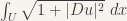
![F[u] = \int_U L(Du,u,x)~dx,](https://s0.wp.com/latex.php?latex=F%5Bu%5D+%3D+%5Cint_U+L%28Du%2Cu%2Cx%29%7Edx%2C&bg=f7f3ee&fg=333333&s=0&c=20201002)
 , then Du is an n x m matrix (though for a real valued u, i.e. where n =1, it is customary to write Du as a row vector, column vectors being hell for typesetting).
![u: [0,1] \to \mathbb{R}](https://s0.wp.com/latex.php?latex=u%3A+%5B0%2C1%5D+%5Cto+%5Cmathbb%7BR%7D&bg=f7f3ee&fg=333333&s=0&c=20201002) which minimizes
which minimizes  , subject to u(0) = a, u(1) = b.

 .
. .
.


 part of the integrand. In fact, if you name any very small number
  , we can choose a member of this sequence so the integral that is smaller than
  . But there is no function where the integral of this Lagrangian is zero, so there is no minimizing function for this particular Lagrangian!


 , for which
  is 1 when j = k, and 0 otherwise, and
  s and c are zero. Put more simply, the Laplacian is the sum of the pure second derivatives. Now we provide first an outline, and then a few details of a proof of existence of solutions.
![B[u,v] = \lambda(v)](https://s0.wp.com/latex.php?latex=B%5Bu%2Cv%5D+%3D+%5Clambda%28v%29&bg=f7f3ee&fg=333333&s=0&c=20201002) for any v, where
for any v, where  is a linear functional (eats functions, gives a number).
 .
.![B[u,v]:=\int\left(\sum_{j,k = 1}^na^{j,k}u_{x_j}v_{x_k}+\sum_{j = 1}^nb^ju_{x_j}v+cuv\right)dx,](https://s0.wp.com/latex.php?latex=B%5Bu%2Cv%5D%3A%3D%5Cint%5Cleft%28%5Csum_%7Bj%2Ck+%3D+1%7D%5Ena%5E%7Bj%2Ck%7Du_%7Bx_j%7Dv_%7Bx_k%7D%2B%5Csum_%7Bj+%3D+1%7D%5Enb%5Eju_%7Bx_j%7Dv%2Bcuv%5Cright%29dx%2C&bg=f7f3ee&fg=333333&s=0&c=20201002)

![B[u,v]=\int Lu\cdot v~dx](https://s0.wp.com/latex.php?latex=B%5Bu%2Cv%5D%3D%5Cint+Lu%5Ccdot+v%7Edx&bg=f7f3ee&fg=333333&s=0&c=20201002) . In this beautiful, integrable, differentiable world, if we could show that
. In this beautiful, integrable, differentiable world, if we could show that  for all functions v, then it would be reasonable to conclude that Lu = f.
 and a (continuous) linear functional
  , there is a unique

![B[u,v]=\lambda(v)](https://s0.wp.com/latex.php?latex=B%5Bu%2Cv%5D%3D%5Clambda%28v%29&bg=f7f3ee&fg=333333&s=0&c=20201002) for each
for each  . There are some other non-trivial hypotheses on B, which may be translated into hypotheses on L, but let’s revel in success now.
 , the m-times differentiable functions- are not Hilbert spaces. Certain Sobolev spaces are, though, and they provide precisely the integrability conditions we need to get precise conditions to guarantee solutions for large classes of PDE.


 , with a Lipschitz function defined on the boundary, is there a “best” Lipschitz function defined on the entire region? By “best”, we’ll mean that on any open bounded subset, the function has the smallest Lipschitz constant given its boundary.
 )
)
 , then write it using Leibniz notation (which is more precise, at the expense of being somewhat intimidating… a topic for another time!) as


 , so
, so  (which again is some formalism that I will duck for now).
 , where the diagonal of J is the [are the?] eigenvalues of A, and then recalling that the determinant of a product is a product of determinants, so
  , and that the trace of similar matrices is the same.) However, Jordan normal form comes, necessarily, later than eigenvalues, and I have never had time to go back to present a complete proof.