Volume of Balls

I like the following question:

“Which dimension has the ‘biggest’ unit ball?”

To define a few words, a “ball” of radius r about a point x in a metric space X with metric d (in particular, in $R^n$ with standard metric) is defined by $B_X(x,r) = \{ y \in X: d(x,y) \leq r \}$ . So the unit ball in Euclidean space is the collection of points of distance less or equal to one from, say, the origin. If you think I am being overly careful with this definition, you’re right!

1-, 2-, and 3-dimensional balls.

By “biggest”, I will mean the n-dimensional volume. So if we define V(n) to be the volume of the unit ball in $R^n$ , then V(1) = 2 (the 1-dimensional ball is a line), $V(2) = \pi r^2 \approx 3.14$ , and $V(3) = \frac{4}{3} \pi r^3 \approx 4.19$ . So the volumes are getting bigger, and maybe we have a good question on our hands. But now what’s the volume of a four dimensional sphere?

It turns out that one can derive the formula

$V(n) = \frac{\pi^{n/2}}{\Gamma(n/2+1)}$ ,

where $\Gamma$ is the gamma function, a generalization of the factorial (!) function! In particular, $\Gamma(n+1) = n!$ for integers n. Then, for even dimensions,

$V(2n) = \frac{\pi^{n}}{n!}$ .

Now so long as we are only worried about integer dimensions, we can use the half-integer identity for the gamma function:
$\Gamma(n+1/2) = \frac{(2n)!}{4^nn!}\sqrt{\pi},$
to get a similar formula for odd dimensions:
$V(2n-1) = \frac{4^n\pi^{n-1}n!}{(2n)!}$ .

Then a quick calculation gives:

V(1) = 2.00
V(2) = 3.14
V(3) = 4.19
V(4) = 4.93
V(5) = 5.26
V(6) = 5.17
V(7) = 4.72
V(8) = 4.06
V(9) = 3.30.

We note that the denominator for both odd and even dimensions grows much faster than the numerator to conclude (in academia we could only nod our head suggestively so far at this conclusion, but we’re in industry now!) that the 5-dimensional ball has the most volume.

As an aside, and possibly a subject for a later post, if we allow for fractional dimensions (everything in V(n) is defined for n a real number, not just an integer), then the maximum value of V is at about 5.2569, where the unit ball has volume around 5.2778.

The function V(n), plotted for real numbers n, with max around (5.26, 5.28).

Math-ing the place up

Mar8

A convex function, with one secant line drawn in red.

Haven’t had a straight up “math” day in quite a while here. That ends now. While reading an article [PDF link], I came across the definition of a Young function: a function $F: [0,\infty) \to [0,\infty)$ which is convex and where F(t) = 0 only when t = 0. Recall that for a real valued function, convex means that every secant line lies above the curve. So far, so good. Such a function might serve as a measure of how alike two functions are: rather than looking at (for example) the $L^2$ norm of u-v, we might first see what we can say about F(|u-v|), a more general question.

But here’s the proposition that made me pause: For 1<q<m<p, there is a differentiable Young function F and a constant C(m,p,q)>0 so that

1. $\int_0^{\infty}F'(t)^{-\frac{1}{m-1}}~dt\leq C$ , and

2. $q\leq \frac{tF'(t)}{F(t)}\leq p$ for all t > 0.

A non-convex function, with a secant line drawn in passing beneath the function.

In fact, there was one more somewhat technical, but non-trivial assertion about this F (proposition 2.1 in the linked paper), but let’s focus on these two. Initially I was convinced that no such F existed, even satisfying these two conditions. Here’s how my erroneous thoughts went: suppose such an F were to exist. Property 2 gives us then that $\frac{qF(t)}{t} \leq F'(t)$ . Solving this “differential inequality” gives us that $F(t) \geq A_1t^q$ . A similar calculation will also yield that $F(t) \leq A_2t^p$ .

Now as a “back of the envelope” calculation, I tried plugging the bounds of F into property 1. Specifically, first I computed

$\int_0^{\infty} A_1qt^{\frac{q-1}{m-1}}dt$ .

Since q<m, the exponent is (strictly) smaller than 1, and the integral diverges (the indefinite integral looks like $ct^{\alpha}$ , where $0<\alpha < 1$ ). In particular, it does great from 0 to any finite number, but has a “fat tail”. Similarly, the integral $\int_0^{\infty} A_1qt^{\frac{p-1}{m-1}}dt$ diverges, but this time because its singularity near zero is too big (the indefinite integral is the same as the previous one, though now $\alpha < 0$. So this one does great from a very small number to infinity, but ultimately diverges.

Possibly I’ve given away the answer since I have emphasized my mis-steps, but here is an example of a Young function satisfying the first two properties. The trick is to construct the function out of two pieces:

The constructed Young function, near where the two "pieces" join.

$F(t) = c_1 t^q$ for small t, and $F(t) = c_2t^p$ for large t. You can even select $c_1, c_2$ so that the derivative is continuous. Explicitly, suppose m = 3. Then we may set F(t) = t for t < 1, and $F(t) = \frac{t^5+4}{5}$ for $t\geq 1$ . Notice that F(t) is continuously differentiable, and that $\int_0^{\infty}F'(t)^{-\frac{1}{m-1}}~dt = 2+1 = 3$ , so we know that $C(3,1,5) \geq 3$ .

Busy days.

Feb29

Somehow spring break has turned into one of the busier weeks of my year. Trying to keep up with real life work has not left a ton of time for writing anything thoughtful/reasonable, though at least for continuity I will try to keep a paragraph or so up here each day with my favorite thought of the day. This also means I can reuse some old graphics!

Today I really enjoyed a particular fact about Sobolev functions. Recall that these are actually equivalence classes of functions, as they are really defined under an integral sign, which “can’t see” sets of small measure. However, the following quantifies exactly how small the bad set might have to be:

If $f \in W^{1,p}(\Omega)$ for $\Omega \subset \mathbb{R}^n$ , then the limit $\lim_{r \to 0} \frac{1}{\alpha(n)r^n}\int_{B(x,r)}f(y)~dy$ exists for all x outside a set E with $\mathcal{H}^{n-p+\epsilon}(E) = 0$ for all $\epsilon > 0$ .

Put another way, every Sobolev function may be “precisely defined” outside a set of small dimension, where the dimension gets smaller as p gets larger. I suppose a given representative may be worse, but this allows you to require that the member of the equivalence class of Sobolev functions has some nice properties.

The fibers of two functions in a sequence. I was thinking the above argument might imply that the limit was not Sobolev, but the limit is precisely represented outside a set with positive 1-dimensional measure, so the result is silent on this issue.

How to solve a variational problem, II

Feb7

Lots of text today = lots of filler photos. Some ducks from the park next door to Rice.

This is a method used to show that a minimizer exists for a variational problem, though it typically provides no clues as to what the minimizer is. It is typically referred to as “the direct method in the calculus of variations”. See yeseterday’s post, at least the first paragraph or two, for background.

First, a point I forgot about yesterday since it is such a convention: “why minimization?” I would guess this is motivated by physics, and has been explored by Hildebrandt and Tromba in The Parsimonious Universe– roughly, that nature seeks to minimize (rather than maximize) energy spent. So much of math has been motivated by physics (often useful, as it provides an intuition as to what should be true), it is only natural many of our questions are posed in this manner. This parsimony can also explain why we typically make sure that the Lagrangian is nonnegative- since energy is nonnegative.

From xkcd. We take the second path here.

Now, the direct method, along with intuition of how we find a least area surface given a prescribed boundary, and what could go wrong in general. We denote the area of a surface u by F[u]:

Geometry? A bridge in upstate New York?

Show that there is at least one candidate minimizer. For the least area surface, we pick a point not on the boundary, and draw a straight line from that point to each boundary point to make our first candidate. As a silly example of what could go wrong, consider trying to minimize the integral of |u|, subject to u(0) = 1 and u(0) = 2. Well, we just cannot satisfy that boundary condition with any function.

2. Take an infimum. We now have a nonempty set of candidates $\{ u_{\alpha} \}$ , which is associated with a nonempty set of real numbers $\{F[u_{\alpha}]\}$ . Going back to the physics explanation, I’ll assume that the integrand is bounded below by zero, and invoke a property of the real numbers to say that there is a greatest lower bound. It will be our goal to find a surface realizing this infimum. Notice though that this step is not constructive, so right here we lose our chance at finding a minimizer analytically. Really the only thing that could go wrong is if our integrand is not bounded below. It would be somewhat silly to try to find the function whose integral is the “most negative”.

Once we have an infimum, M, we can take a sequence of candidates $\{u_j\}$ which converge to the infimum, $F[u_j] \to M$ . Notice that the candidate functions do not necessarily converge to anything. Yet.

"Bikeman" in some of the most beautiful woods in the world.

3. Invoke compactness. Now, lurking under the surface has been this “space of admissible functions”. Often this is a Sobolev space, which has the property that the unit ball is “(weak-*) compact”. See this short paper (pdf link) by Frank Morgan on compactness, which he called “the most important concept in mathematics”. Compactness implies that every bounded sequence has a convergent subsequence. Here “bounded” means “with respect to the norm on the space”. In the case of area minimizers, there is a “mass norm” on the admissible functions (“integer rectifiable currents”) which measures the surface area, and a famous (for some value of the word “famous”) compactness theorem for these functions (defining a space of admissible functions that was physically relevant and so that such a theorem existed was, perhaps, the most difficult part of Plateau’s problem). Hence, we now have a subsequence $\{u_{j'} \}$ , and a target (admissible) function u so that $u_{j'} \to u$ and $F[u_{j'}] \to M$ , still.

A sequence of functions converging to the infimum for the integral of |u(x)| subject to u(0) = 0, u(1) = 1. However, there is no smooth function that they are converging to. This sequence appears on the cover of Frank Morgan's real analysis text.

Last thing to show is that F[u] = M. The two conditions we’ve established certainly nod suggestively at this last equation, but don’t give it themselves. The figure at right shows what could go wrong.

4. Lower semicontinuity of the functional. We need to show that F[u] = M. A typical approach is to prove that the functional is lower semicontinuous. That is to say, $F[\liminf u_j] \leq \liminf F[u_j]$ (fun story: when I asked my advisor to define “upper semicontinuity”, he gave me the finger. Bonus points if you can see why this is a reasonable definition). If this is true, then we have $M \leq F[u] = F[\liminf u_j] \leq \liminf F[u_j] = M$ , and are done. The surface area is lower semicontinuous, which is how we complete the proof of the existence of area minimizing surfaces.

Reusing figures! Non lowersemicontinuity.

The Takagi curves from yesterday provide an example of a functional which is not lower semicontinuous, since $F[u_j] \to 0$ , but $F[u] = 1$ .

How to solve a variational problem, I

Feb6

Only had 5 figures and 600 words, so here's a photo of a saddle in the Guadalupe Mountains. I like that you can see all the "local maxima" easily. If you look closely, you can even see a trail crossing right at the lowest point of the saddle.

Last week, I discussed how to solve a PDE. This week, I want to talk about how to solve a variational problem. By variational problem, I will mean minimizing an integral like

$F[u] = \int_U L(Du,u,x)~dx,$

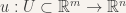
subject to some boundary conditions, where U is a subset of some Euclidean space, u is the function we are solving for (which maps from U to some other Euclidean space), and Du is the differential of u. If $u: U \subset \mathbb{R}^m \to \mathbb{R}^n$ , then Du is an n x m matrix (though for a real valued u, i.e. where n =1, it is customary to write Du as a row vector, column vectors being hell for typesetting).

Today I focus on examples of variational problems which can be solved analytically, while tomorrow will be an outline of the so-called “direct method in the calculus of variations”.

One minimizer of the integral of u'(x). Any function would do.

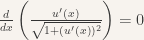
First, a variational problem which is (hopefully) easily solved by any student of calculus: Find a function $u: [0,1] \to \mathbb{R}$ which minimizes $\int_0^1 u'(x)~dx$ , subject to u(0) = a, u(1) = b.

In this case, we know that any function that starts at a and ends at b will be a minimizer, since, by the fundamental theorem of calculus,

$\int_0^1u'(x)~dx = u(1)-u(0) = b-a.$

Hence, we have existence, but not uniqueness.

The most famous variational problem is surely minimizing surface area (or length, or volume depending on the dimension of the domain) of a graph. That is, finding a real valued function u that minimizes

$\int_U \sqrt{1+|Du|^2}~dx$

subject to some boundary conditions.

The *only* function that minimizes length, with u(0) = a, u(1) = b.

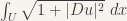
Longtime reader(s) will recall the Euler-Lagrange equationswhich can sometimes provide a solution to such problems:

$\left. D_uL(Du,u,x)-div_x(D_pL(Du,u,x))=0 \right.$ .

As an easy example, if we wanted to minimize the length of a line, we would use the above functional, Du = u’ in this case (the ol’ 1 x 1 matrix), and the Euler-Lagrange equations give

$\frac{d}{dx}\left( \frac{u'(x)}{\sqrt{1+(u'(x))^2}} \right) = 0$ .

Rather than calculate this derivative, we notice that this means

$\frac{u'(x)}{\sqrt{1+(u'(x))^2}} = C$

$u'(x) = \frac{C}{\sqrt{1- C^2}} = D.$

Hence, u’ is a constant, and our solution must be a straight line, u(x) = Dx+E.

We also point out that it should be surprising that there are any general results for solving variational problems. This post was inspired by Leonid Kovalev’s discussion of the Takagi curve, which is a fractal whose iterates look like a famous counterexample. Specifically, suppose we wish to minimize

$\int_0^1 u(x)^2+(1-|u'(x)|)^2~dx,$

subject to u(0) = u(1) = 0. Notice that the integrand is

Takagi curves

Always nonnegative,
small when u is close to 0,
small when u’ is close to +1 or -1,
only 0 if u is (almost) always 0 and |u’| is (almost) always plus or minus 1.

The sequence of functions pictured at the bottom of the post (which forms the Takagi curve) will always have 0 for the derivative part, and will be getting smaller and smaller on the $u(x)^2$ part of the integrand. In fact, if you name any very small number $\epsilon > 0$ , we can choose a member of this sequence so the integral that is smaller than $\epsilon$ . But there is no function where the integral of this Lagrangian is zero, so there is no minimizing function for this particular Lagrangian!

A sequence of functions, where the integrals of the Lagrangians converge to zero, but there is no limit where the integral of the Lagrangian is zero.

As an aside, I’m sure that this Lagrangian is named/famous, but I could not find mention of it in any of my usual sources…

MATLAB code to generate the above gif. Remove the “pause” commands to just plot everything at once:
function takcurves(n) %generates n iterates of the Takagi curves ColOrd = hsv(n); figure(1) set(gcf, 'Position', get(0,'Screensize')); hold on pause(0.4) for j = 1:n x = 0:.5^j:1; y = zeros(size(x)); y(2:2:size(y,2)) = .5^j; line(x,y,'LineSmoothing','on','Color',ColOrd(j,:)) hold on pause(0.4) end hold off end

More geometry with inverse images

Feb1

Yesterday’s post was on inverse images of functions as sets, and ways to visualize them. Today, I realized that despite my early series of posts on the Jacobian derailing, I probably have enough background to describe the area and coarea formulae. The two give a relationship between the “size” of the fibers and the derivative of the map. The first thing I’ll need to do is define the Jacobian for maps $f: \mathbb{R}^m \to \mathbb{R}^n$ . The definition will be slightly different depending on whether m or n is larger, but if $n \geq m$ , then

$|Jf(x)| := \sqrt{|Df(x)^T \cdot Df(x)|}$ ,

and if $m \geq n$ , then

$|Jf(x)| := \sqrt{|Df(x) \cdot Df(x)^T|}$

where Df is the n x m matrix of partial derivatives of f, and we use the absolute value bars to indicate a determinant. Notice that if m = n, then the definitions agree, and it is just the absolute value of the determinant of the matrix of partial derivatives. If n = 1 so that f is a real-valued function, then the Jacobian is the length of the gradient of f.

Now then, the area formula says that for a Lipschitz $f:\mathbb{R}^m \to \mathbb{R}^n$ with $m \leq n$ , and any Lebesgue measurable $U \subset \mathbb{R}^m$ ,

$\int_U |Jf(x)| d\mathcal{L}^m(x) = \int_{\mathbb{R}^n} \#(f^{-1}(y) \cap U)~d\mathcal{H}^m(y),$

A hyperboloid projecting onto a circle.

where, for a set S, $\#(S)$ denotes the cardinality of S, i.e., how many points are in S. We expect this number to be finite (for most functions f I think of, each inverse image has cardinality either 1 or 0). Indeed, notice that if f is a smooth embedding, then f is one-to-one, and the right hand side of the above is always 1 if f maps there. Hence the right hand side will be $\mathcal{H}^m(f(U))$ , the area of the image of U under f. This explains why it is called the area formula- it agrees with the classical area of parametrized surfaces.

The coarea formula (the subject of my research) keeps all the conditions above, but now f maps from high dimensions into a lower one, so $m \geq n$ . We have

$\int_U |Jf(x)| d\mathcal{L}^m(x) = \int_{\mathbb{R}^n} \mathcal{H}^{m-n}(f^{-1}(y) \cap U)~d\mathcal{H}^n(y).$

In plain English, the integral of the Jacobian of f is equal to the integral of the length of the fibers of f. [Technical sentences coming up!] One surprising fact is that this coarea formula was first proven in 1959 in Herbert Federer’s paper “Curvature Measures“, while the area formula was (is) a basic calculus fact, at least for smooth functions. The formula has since played a role in image processing, as when f is a real valued function, the quantity is usually referred to as the total variation. De Giorgi showed that the fibers of functions which minimized the left hand side are actually minimal surfaces.

A string hyperboloid.

I’ve included a few illustrations of how the coarea formula might relate to “projections” of hyperboloids onto the circle. The first shows such a hyperboloid, along with the fibers of the “projection”. The coarea of this map will be the surface area of the hyperboloid. Such a hyperboloid can be made with string from a cylinder, and twisting the top. See the second figure. The final .gif illustrates continuing to twist the top, and the resulting surfaces. In each case, integrating the function whose level sets are these straight lines will return the surface area of the hyperboloid

Twisting hyperboloids

Hausdorff dimension II

Jan24

I left off yesterday asking how to measure a surface (something sort of 2-dimensional) in 3-space, and noting that Lebesgue measure would give this set 0 area. This is where Hausdorff measure comes in. There is in fact a continuum of Hausdorff measures, one for each real number. First it is helpful to define the diameter of a set, which is just the farthest distance apart of two points in the set. For a circle, the diameter is the usual definition. Also, we’ll denote the diameter of a set U by |U|.

The construction of the measure is typically described in two steps: Suppose we are trying to find the m-dimensional Hausdorff measure of a set U. Then in the first step, we cover U by sets no larger than some number, d, and look at the sum of the diameters of these sets raised to the mth power. The smallest (well, infimum) of these coverings will be the number we associate with the parameter d. In the second step, we let d go to zero. The Hausdorff measure is the limit, if it exists. In symbols,

: Two sets with (approximately) the same diameter, indicated with the red line.

$H^m_d(U) = inf \sum_{k = 1}^{\infty} |U_k|^m$ , where $|U_k| < d$ for each k. Then $H^m(U) = \lim_{d \to 0} H^m_d(U)$ . There is an easy result (see, for example, Falconer’s “Geometry of Fractal Sets“) that says that for any set U, there is a unique value, called the Hausdorff dimension of U so that $H^m(U) = \infty \text{ if } 0 \leq d < \dim U$ and $H^d(E) = 0 \text{ if } \dim U< s < \infty$ . Note that the Hausdorff measure might be 0 or infinite, but this number will still exist.

We should also note that:

Nowhere in the definition did I use anything but distance, making all these concepts valid in metric spaces, as well as in Euclidean (vector) spaces.
Nowhere in the definition did I require the Hausdorff dimension to be an integer.

Expanding on this second point brings us into discussing fractals, which I have discussed a bit in the past week, but have not defined. One reason for this is that I have not seen a great definition. Self similarity is important, as is having a Hausdorff dimension different from its topological dimension. At the very least, any self similar set whose Hausdorff dimension is not an integer would be given “fractal” status, though this would miss many good examples. In any case, for any self similar set, the Hausdorff dimension is log(m)/log(s), where m is the number of copies at each step, and s is the (linear) scaling factor.

So if you view the real plane as a self similar set taken by starting with a square, then dividing it into four squares, and then each of those into four squares, and so on, then the number of copies is 4 and the scaling factor is 2 (Remember, it is the linear scaling factor! Each side is half the length it used to be.), so the Hausdorff dimension is log(4)/log(2), which is precisely 2, since $\log{4}/\log{2} = \log{2^2}/\log{2} = 2\log{2}/\log{2}$ .

I have printed below two more examples of fractals and their dimensions. Thanks to Leonid Kovalev for pointing out how to generate the Sierpinski carpet. Also see this great wikipedia post for a much more complete list of fractals and their dimensions.

: Dimension log(3)/log(2).

: Has dimension log(8)/log(3) = 3*log(2)/log(3).

Introduction to Hausdorff Measure

Jan23

It was not until my third year of graduate school that I thought to ask why geometric measure theory was called geometric measure theory. It just always seemed like the answer should have been fairly obvious- the questions were very geometric, and everyone likes measures, right? Well the prototypical problem in GMT is Plateau’s problem, which is roughly: given a closed curve in three space, what surface has the smallest area, and the given curve as a boundary.

A curve in 3-space, and a minimizing surface.

In order to study this problem for a “large enough” collection of sets to guarantee a solution, mathematicians could not rely on nice parameterizations existing over which surface integrals would be taken. This can be thought of in analogy with the fact that “every nth degree polynomial has n roots” is not true over the real numbers, but it is true over the complex numbers. But the notion of the area of such a “rectifiable set” is not immediately clear.

Covering a set by squares

More precisely, in mathematics, a “measure” is a function which eats sets, and returns a number that is, intuitively, the “size” of that set. Perhaps the most commonly used measure- Lebesgue measure- is constructed exactly in this intuitive manner. We first cover the set with squares (or lines in dimension 1, or cubes in dimension 3, or hypercubes in dimension 4, etc) with side length 1, then squares of side length 0.5, then 0.25, and so on. By adding up the area (the area of an n-cube we define to be the side length to the nth power) of the squares in each case, we get a sequence, and if (when) that sequence converges, we call the number the (Lebesgue) measure of the set.

The problem with this approach is that if I have a reasonable line sitting in the plane, the Lebesgue measure of that line will be 0. Similarly for a surface sitting in 3-space. This is, in some sense, good. The “length” of a point should be 0, and the “area” of a line should also be 0. But this is a bad thing in the sense that maybe someone (like Joseph Plateau) is interested in the area of a surface in 3-space.

Covering the same set with smaller squares.

Tomorrow will be more on finding the area of such a surface (hint: the answer is Hausdorff measure)! And fractals! Then maybe the discussion will come back to “why is it called geometric measure theory?”

Variational thoughts

Thoughts about math or whatever is interesting this day, with a picture every 100 words. Updates M-F.

Category Archives: geometric measure theory