How to solve a variational problem, I

Only had 5 figures and 600 words, so here's a photo of a saddle in the Guadalupe Mountains. I like that you can see all the "local maxima" easily. If you look closely, you can even see a trail crossing right at the lowest point of the saddle.

Last week, I discussed how to solve a PDE.  This week, I want to talk about how to solve a variational problem.  By variational problem, I will mean minimizing an integral like

subject to some boundary conditions, where U is a subset of some Euclidean space,  u is the function we are solving for (which maps from U to some other Euclidean space), and Du is the differential of u.  If 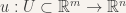, then Du is an n x m matrix (though for a real valued u, i.e. where n =1, it is customary to write Du as a row vector, column vectors being hell for typesetting).

Today I focus on examples of variational problems which can be solved analytically, while tomorrow will be an outline of the so-called “direct method in the calculus of variations”.

One minimizer of the integral of u'(x). Any function would do.

First, a variational problem which is (hopefully) easily solved by any student of calculus: Find a function which minimizes , subject to u(0) = a, u(1) = b.

In this case, we know that any function that starts at a and ends at b will be a minimizer, since, by the fundamental theorem of calculus,

Hence, we have existence, but not uniqueness.

The most famous variational problem is surely minimizing surface area (or length, or volume depending on the dimension of the domain) of a graph.  That is, finding a real valued function u that minimizes

subject to some boundary conditions.

The *only* function that minimizes length, with u(0) = a, u(1) = b.

Longtime reader(s) will recall the Euler-Lagrange equationswhich can sometimes provide a solution to such problems:

.

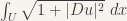
As an easy example, if we wanted to minimize the length of a line, we would use the above functional, Du = u’ in this case (the ol’ 1 x 1 matrix), and the Euler-Lagrange equations give

.

Rather than calculate this derivative, we notice that this means

so

Hence, u’ is a constant, and our solution must be a straight line, u(x) = Dx+E.

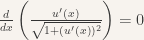
We also point out that it should be surprising that there are any general results for solving variational problems.  This post was inspired by Leonid Kovalev’s discussion of the Takagi curve, which is a fractal whose iterates look like a famous counterexample.  Specifically, suppose we wish to minimize

subject to u(0) = u(1) = 0.  Notice that the integrand is

1. 

   Takagi curves

   Always nonnegative,

2. small when u is close to 0,
3. small when u’ is close to +1 or -1,
4. only 0 if u is (almost) always 0 and |u’| is (almost) always plus or minus 1.

The sequence of functions pictured at the bottom of the post (which forms the Takagi curve) will always have 0 for the derivative part, and will be getting smaller and smaller on the part of the integrand.  In fact, if you name any very small number , we can choose a member of this sequence so the integral that is smaller than .  But there is no function where the integral of this Lagrangian is zero, so there is no minimizing function for this particular Lagrangian!

A sequence of functions, where the integrals of the Lagrangians converge to zero, but there is no limit where the integral of the Lagrangian is zero.

As an aside, I’m sure that this Lagrangian is named/famous, but I could not find mention of it in any of my usual sources…

MATLAB code to generate the above gif.  Remove the “pause” commands to just plot everything at once:

function takcurves(n)
%generates n iterates of the Takagi curves
ColOrd = hsv(n);
figure(1)
set(gcf, 'Position', get(0,'Screensize'));
hold on
pause(0.4)
for j = 1:n
x = 0:.5^j:1;
y = zeros(size(x));
y(2:2:size(y,2)) = .5^j;
line(x,y,'LineSmoothing','on','Color',ColOrd(j,:))
hold on
pause(0.4)
end
hold off
end